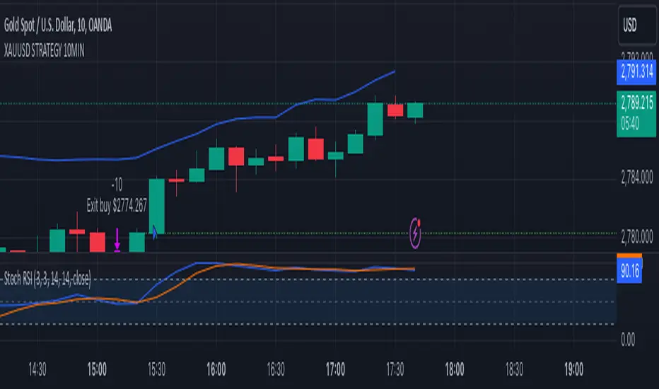
XAUUSD 10-Minute StrategyThis XAUUSD 10-Minute Strategy is designed for trading Gold vs. USD on a 10-minute timeframe. By combining multiple technical indicators (MACD, RSI, Bollinger Bands, and ATR), the strategy effectively captures both trend-following and reversal opportunities, with adaptive risk management for varying market volatility. This approach balances high-probability entries with robust volatility management, making it suitable for traders seeking to optimise entries during significant price movements and reversals.
Key Components and Logic:
MACD (12, 26, 9):
Generates buy signals on MACD Line crossovers above the Signal Line and sell signals on crossovers below the Signal Line, helping to capture momentum shifts.
RSI (14):
Utilizes oversold (below 35) and overbought (above 65) levels as a secondary filter to validate entries and avoid overextended price zones.
Bollinger Bands (20, 2):
Uses upper and lower Bollinger Bands to identify potential overbought and oversold conditions, aiming to enter long trades near the lower band and short trades near the upper band.
ATR-Based Stop Loss and Take Profit:
Stop Loss and Take Profit levels are dynamically set as multiples of ATR (3x for stop loss, 5x for take profit), ensuring flexibility with market volatility to optimise exit points.
Entry & Exit Conditions:
Buy Entry: T riggered when any of the following conditions are met:
MACD Line crosses above the Signal Line
RSI is oversold
Price drops below the lower Bollinger Band
Sell Entry: Triggered when any of the following conditions are met:
MACD Line crosses below the Signal Line
RSI is overbought
Price moves above the upper Bollinger Band
Exit Strategy: Trades are closed based on opposing entry signals, with adaptive spread adjustments for realistic exit points.
Backtesting Configuration & Results:
Backtesting Period: July 21, 2024, to October 30, 2024
Symbol Info: XAUUSD, 10-minute timeframe, OANDA data source
Backtesting Capital: Initial capital of $700, with each trade set to 10 contracts (equivalent to approximately 0.1 lots based on the broker’s contract size for gold).
Users should confirm their broker's contract size for gold, as this may differ. This script uses 10 contracts for backtesting purposes, aligned with 0.1 lots on brokers offering a 100-contract specification.
Key Backtesting Performance Metrics:
Net Profit: $4,733.90 USD (676.27% increase)
Total Closed Trades: 526
Win Rate: 53.99%
Profit Factor: 1.44 (1.96 for Long trades, 1.14 for Short trades)
Max Drawdown: $819.75 USD (56.33% of equity)
Sharpe Ratio: 1.726
Average Trade: $9.00 USD (0.04% of equity per trade)
This backtest reflects realistic conditions, with a spread adjustment of 38 points and no slippage or commission applied. The settings aim to simulate typical retail trading conditions. However, please adjust the initial capital, contract size, and other settings based on your account specifics for best results.
Usage:
This strategy is tuned specifically for XAUUSD on a 10-minute timeframe, ideal for both trend-following and reversal trades. The ATR-based stop loss and take profit levels adapt dynamically to market volatility, optimising entries and exits in varied conditions. To backtest this script accurately, ensure your broker’s contract specifications for gold align with the parameters used in this strategy.
Cari dalam skrip untuk "the strat"
Up/Down Volume with Normal DistributionThis indicator analyzes the relationship between price movements and trading volume by distinguishing between "up" and "down" volume. Up volume refers to trading volume occurring during price increases, while down volume refers to trading volume during price decreases. The indicator calculates the mean and standard deviation for both up and down volume over a specified length. This statistical approach enables traders to visualize volume deviations from the average, highlighting potential market anomalies that could signal trading opportunities.
Relationship Between Price and Volume
Volume is a critical metric in technical analysis, often considered a leading indicator of price movements. According to studies in financial economics, significant price changes accompanied by high volume tend to indicate strong market conviction (Wyart et al., 2008). Conversely, price changes on low volume may suggest a lack of interest or conviction, making those moves less reliable.
The relationship between price and volume can be summarized as follows:
Confirmation of Trends: High volume accompanying a price increase often confirms an upward trend. Similarly, high volume during price declines indicates bearish sentiment.
Reversals and Exhaustion: Decreases in volume during price increases may suggest a potential reversal or exhaustion of buying pressure, while increased volume during declines can indicate capitulation.
Breakouts: Price movements that break through significant resistance or support levels accompanied by high volume are typically more significant and suggest stronger follow-through in the new direction.
Developing a Trading Strategy
Traders can leverage the insights gained from this relationship to formulate a trading strategy based on volume analysis:
Entry Signals: Traders can enter long positions when the up volume significantly exceeds the mean by a predefined number of standard deviations. This situation indicates strong buying interest. Conversely, short positions can be initiated when down volume exceeds the mean by a specified standard deviation.
Exit Signals: Exiting positions can be based on changes in volume patterns. If the volume starts to decrease significantly after a price increase, this may signal a potential reversal or the need to lock in profits.
Risk Management: Integrating volume analysis with other technical indicators, such as moving averages or RSI, can provide a more comprehensive risk management framework, enhancing the overall effectiveness of the strategy.
In conclusion, understanding the relationship between price and volume, alongside employing statistical measures like the mean and standard deviation, enables traders to create more robust trading strategies that capitalize on market movements.
References
Wyart, M., Bouchaud, J.-P., & Dacorogna, M. (2008). "Self-organized volatility in a complicated market." European Physical Journal B, 61(2), 195-203. doi:10.1140

ICT Master Suite [Trading IQ]Hello Traders!
We’re excited to introduce the ICT Master Suite by TradingIQ, a new tool designed to bring together several ICT concepts and strategies in one place.
The Purpose Behind the ICT Master Suite
There are a few challenges traders often face when using ICT-related indicators:
Many available indicators focus on one or two ICT methods, which can limit traders who apply a broader range of ICT related techniques on their charts.
There aren't many indicators for ICT strategy models, and we couldn't find ICT indicators that allow for testing the strategy models and setting alerts.
Many ICT related concepts exist in the public domain as indicators, not strategies! This makes it difficult to verify that the ICT concept has some utility in the market you're trading and if it's worth trading - it's difficult to know if it's working!
Some users might not have enough chart space to apply numerous ICT related indicators, which can be restrictive for those wanting to use multiple ICT techniques simultaneously.
The ICT Master Suite is designed to offer a comprehensive option for traders who want to apply a variety of ICT methods. By combining several ICT techniques and strategy models into one indicator, it helps users maximize their chart space while accessing multiple tools in a single slot.
Additionally, the ICT Master Suite was developed as a strategy . This means users can backtest various ICT strategy models - including deep backtesting. A primary goal of this indicator is to let traders decide for themselves what markets to trade ICT concepts in and give them the capability to figure out if the strategy models are worth trading!
What Makes the ICT Master Suite Different
There are many ICT-related indicators available on TradingView, each offering valuable insights. What the ICT Master Suite aims to do is bring together a wider selection of these techniques into one tool. This includes both key ICT methods and strategy models, allowing traders to test and activate strategies all within one indicator.
Features
The ICT Master Suite offers:
Multiple ICT strategy models, including the 2022 Strategy Model and Unicorn Model, which can be built, tested, and used for live trading.
Calculation and display of key price areas like Breaker Blocks, Rejection Blocks, Order Blocks, Fair Value Gaps, Equal Levels, and more.
The ability to set alerts based on these ICT strategies and key price areas.
A comprehensive, yet practical, all-inclusive ICT indicator for traders.
Customizable Timeframe - Calculate ICT concepts on off-chart timeframes
Unicorn Strategy Model
2022 Strategy Model
Liquidity Raid Strategy Model
OTE (Optimal Trade Entry) Strategy Model
Silver Bullet Strategy Model
Order blocks
Breaker blocks
Rejection blocks
FVG
Strong highs and lows
Displacements
Liquidity sweeps
Power of 3
ICT Macros
HTF previous bar high and low
Break of Structure indications
Market Structure Shift indications
Equal highs and lows
Swings highs and swing lows
Fibonacci TPs and SLs
Swing level TPs and SLs
Previous day high and low TPs and SLs
And much more! An ongoing project!
How To Use
Many traders will already be familiar with the ICT related concepts listed above, and will find using the ICT Master Suite quite intuitive!
Despite this, let's go over the features of the tool in-depth and how to use the tool!
The image above shows the ICT Master Suite with almost all techniques activated.
ICT 2022 Strategy Model
The ICT Master suite provides the ability to test, set alerts for, and live trade the ICT 2022 Strategy Model.
The image above shows an example of a long position being entered following a complete setup for the 2022 ICT model.
A liquidity sweep occurs prior to an upside breakout. During the upside breakout the model looks for the FVG that is nearest 50% of the setup range. A limit order is placed at this FVG for entry.
The target entry percentage for the range is customizable in the settings. For instance, you can select to enter at an FVG nearest 33% of the range, 20%, 66%, etc.
The profit target for the model generally uses the highest high of the range (100%) for longs and the lowest low of the range (100%) for shorts. Stop losses are generally set at 0% of the range.
The image above shows the short model in action!
Whether you decide to follow the 2022 model diligently or not, you can still set alerts when the entry condition is met.
ICT Unicorn Model
The image above shows an example of a long position being entered following a complete setup for the ICT Unicorn model.
A lower swing low followed by a higher swing high precedes the overlap of an FVG and breaker block formed during the sequence.
During the upside breakout the model looks for an FVG and breaker block that formed during the sequence and overlap each other. A limit order is placed at the nearest overlap point to current price.
The profit target for this example trade is set at the swing high and the stop loss at the swing low. However, both the profit target and stop loss for this model are configurable in the settings.
For Longs, the selectable profit targets are:
Swing High
Fib -0.5
Fib -1
Fib -2
For Longs, the selectable stop losses are:
Swing Low
Bottom of FVG or breaker block
The image above shows the short version of the Unicorn Model in action!
For Shorts, the selectable profit targets are:
Swing Low
Fib -0.5
Fib -1
Fib -2
For Shorts, the selectable stop losses are:
Swing High
Top of FVG or breaker block
The image above shows the profit target and stop loss options in the settings for the Unicorn Model.
Optimal Trade Entry (OTE) Model
The image above shows an example of a long position being entered following a complete setup for the OTE model.
Price retraces either 0.62, 0.705, or 0.79 of an upside move and a trade is entered.
The profit target for this example trade is set at the -0.5 fib level. This is also adjustable in the settings.
For Longs, the selectable profit targets are:
Swing High
Fib -0.5
Fib -1
Fib -2
The image above shows the short version of the OTE Model in action!
For Shorts, the selectable profit targets are:
Swing Low
Fib -0.5
Fib -1
Fib -2
Liquidity Raid Model
The image above shows an example of a long position being entered following a complete setup for the Liquidity Raid Modell.
The user must define the session in the settings (for this example it is 13:30-16:00 NY time).
During the session, the indicator will calculate the session high and session low. Following a “raid” of either the session high or session low (after the session has completed) the script will look for an entry at a recently formed breaker block.
If the session high is raided the script will look for short entries at a bearish breaker block. If the session low is raided the script will look for long entries at a bullish breaker block.
For Longs, the profit target options are:
Swing high
User inputted Lib level
For Longs, the stop loss options are:
Swing low
User inputted Lib level
Breaker block bottom
The image above shows the short version of the Liquidity Raid Model in action!
For Shorts, the profit target options are:
Swing Low
User inputted Lib level
For Shorts, the stop loss options are:
Swing High
User inputted Lib level
Breaker block top
Silver Bullet Model
The image above shows an example of a long position being entered following a complete setup for the Silver Bullet Modell.
During the session, the indicator will determine the higher timeframe bias. If the higher timeframe bias is bullish the strategy will look to enter long at an FVG that forms during the session. If the higher timeframe bias is bearish the indicator will look to enter short at an FVG that forms during the session.
For Longs, the profit target options are:
Nearest Swing High Above Entry
Previous Day High
For Longs, the stop loss options are:
Nearest Swing Low
Previous Day Low
The image above shows the short version of the Silver Bullet Model in action!
For Shorts, the profit target options are:
Nearest Swing Low Below Entry
Previous Day Low
For Shorts, the stop loss options are:
Nearest Swing High
Previous Day High
Order blocks
The image above shows indicator identifying and labeling order blocks.
The color of the order blocks, and how many should be shown, are configurable in the settings!
Breaker Blocks
The image above shows indicator identifying and labeling order blocks.
The color of the breaker blocks, and how many should be shown, are configurable in the settings!
Rejection Blocks
The image above shows indicator identifying and labeling rejection blocks.
The color of the rejection blocks, and how many should be shown, are configurable in the settings!
Fair Value Gaps
The image above shows indicator identifying and labeling fair value gaps.
The color of the fair value gaps, and how many should be shown, are configurable in the settings!
Additionally, you can select to only show fair values gaps that form after a liquidity sweep. Doing so reduces "noisy" FVGs and focuses on identifying FVGs that form after a significant trading event.
The image above shows the feature enabled. A fair value gap that occurred after a liquidity sweep is shown.
Market Structure
The image above shows the ICT Master Suite calculating market structure shots and break of structures!
The color of MSS and BoS, and whether they should be displayed, are configurable in the settings.
Displacements
The images above show indicator identifying and labeling displacements.
The color of the displacements, and how many should be shown, are configurable in the settings!
Equal Price Points
The image above shows the indicator identifying and labeling equal highs and equal lows.
The color of the equal levels, and how many should be shown, are configurable in the settings!
Previous Custom TF High/Low
The image above shows the ICT Master Suite calculating the high and low price for a user-defined timeframe. In this case the previous day’s high and low are calculated.
To illustrate the customizable timeframe function, the image above shows the indicator calculating the previous 4 hour high and low.
Liquidity Sweeps
The image above shows the indicator identifying a liquidity sweep prior to an upside breakout.
The image above shows the indicator identifying a liquidity sweep prior to a downside breakout.
The color and aggressiveness of liquidity sweep identification are adjustable in the settings!
Power Of Three
The image above shows the indicator calculating Po3 for two user-defined higher timeframes!
Macros
The image above shows the ICT Master Suite identifying the ICT macros!
ICT Macros are only displayable on the 5 minute timeframe or less.
Strategy Performance Table
In addition to a full-fledged TradingView backtest for any of the ICT strategy models the indicator offers, a quick-and-easy strategy table exists for the indicator!
The image above shows the strategy performance table in action.
Keep in mind that, because the ICT Master Suite is a strategy script, you can perform fully automatic backtests, deep backtests, easily add commission and portfolio balance and look at pertinent metrics for the ICT strategies you are testing!
Lite Mode
Traders who want the cleanest chart possible can toggle on “Lite Mode”!
In Lite Mode, any neon or “glow” like effects are removed and key levels are marked as strict border boxes. You can also select to remove box borders if that’s what you prefer!
Settings Used For Backtest
For the displayed backtest, a starting balance of $1000 USD was used. A commission of 0.02%, slippage of 2 ticks, a verify price for limit orders of 2 ticks, and 5% of capital investment per order.
A commission of 0.02% was used due to the backtested asset being a perpetual future contract for a crypto currency. The highest commission (lowest-tier VIP) for maker orders on many exchanges is 0.02%. All entered positions take place as maker orders and so do profit target exits. Stop orders exist as stop-market orders.
A slippage of 2 ticks was used to simulate more realistic stop-market orders. A verify limit order settings of 2 ticks was also used. Even though BTCUSDT.P on Binance is liquid, we just want the backtest to be on the safe side. Additionally, the backtest traded 100+ trades over the period. The higher the sample size the better; however, this example test can serve as a starting point for traders interested in ICT concepts.
Community Assistance And Feedback
Given the complexity and idiosyncratic applications of ICT concepts amongst its proponents, the ICT Master Suite’s built-in strategies and level identification methods might not align with everyone's interpretation.
That said, the best we can do is precisely define ICT strategy rules and concepts to a repeatable process, test, and apply them! Whether or not an ICT strategy is trading precisely how you would trade it, seeing the model in action, taking trades, and with performance statistics is immensely helpful in assessing predictive utility.
If you think we missed something, you notice a bug, have an idea for strategy model improvement, please let us know! The ICT Master Suite is an ongoing project that will, ideally, be shaped by the community.
A big thank you to the @PineCoders for their Time Library!
Thank you!

Ultimate Oscillator Trading StrategyThe Ultimate Oscillator Trading Strategy implemented in Pine Script™ is based on the Ultimate Oscillator (UO), a momentum indicator developed by Larry Williams in 1976. The UO is designed to measure price momentum over multiple timeframes, providing a more comprehensive view of market conditions by considering short-term, medium-term, and long-term trends simultaneously. This strategy applies the UO as a mean-reversion tool, seeking to capitalize on temporary deviations from the mean price level in the asset’s movement (Williams, 1976).
Strategy Overview:
Calculation of the Ultimate Oscillator (UO):
The UO combines price action over three different periods (short-term, medium-term, and long-term) to generate a weighted momentum measure. The default settings used in this strategy are:
Short-term: 6 periods (adjustable between 2 and 10).
Medium-term: 14 periods (adjustable between 6 and 14).
Long-term: 20 periods (adjustable between 10 and 20).
The UO is calculated as a weighted average of buying pressure and true range across these periods. The weights are designed to give more emphasis to short-term momentum, reflecting the short-term mean-reversion behavior observed in financial markets (Murphy, 1999).
Entry Conditions:
A long position is opened when the UO value falls below 30, indicating that the asset is potentially oversold. The value of 30 is a common threshold that suggests the price may have deviated significantly from its mean and could be due for a reversal, consistent with mean-reversion theory (Jegadeesh & Titman, 1993).
Exit Conditions:
The long position is closed when the current close price exceeds the previous day’s high. This rule captures the reversal and price recovery, providing a defined point to take profits.
The use of previous highs as exit points aligns with breakout and momentum strategies, as it indicates sufficient strength for a price recovery (Fama, 1970).
Scientific Basis and Rationale:
Momentum and Mean-Reversion:
The strategy leverages two well-established phenomena in financial markets: momentum and mean-reversion. Momentum, identified in earlier studies like those by Jegadeesh and Titman (1993), describes the tendency of assets to continue in their direction of movement over short periods. Mean-reversion, as discussed by Poterba and Summers (1988), indicates that asset prices tend to revert to their mean over time after short-term deviations. This dual approach aims to buy assets when they are temporarily oversold and capitalize on their return to the mean.
Multi-timeframe Analysis:
The UO’s incorporation of multiple timeframes (short, medium, and long) provides a holistic view of momentum, unlike single-period oscillators such as the RSI. By combining data across different timeframes, the UO offers a more robust signal and reduces the risk of false entries often associated with single-period momentum indicators (Murphy, 1999).
Trading and Market Efficiency:
Studies in behavioral finance, such as those by Shiller (2003), show that short-term inefficiencies and behavioral biases can lead to overreactions in the market, resulting in price deviations. This strategy seeks to exploit these temporary inefficiencies, using the UO as a signal to identify potential entry points when the market sentiment may have overly pushed the price away from its average.
Strategy Performance:
Backtests of this strategy show promising results, with profit factors exceeding 2.5 when the default settings are optimized. These results are consistent with other studies on short-term trading strategies that capitalize on mean-reversion patterns (Jegadeesh & Titman, 1993). The use of a dynamic, multi-period indicator like the UO enhances the strategy’s adaptability, making it effective across different market conditions and timeframes.
Conclusion:
The Ultimate Oscillator Trading Strategy effectively combines momentum and mean-reversion principles to trade on temporary market inefficiencies. By utilizing multiple periods in its calculation, the UO provides a more reliable and comprehensive measure of momentum, reducing the likelihood of false signals and increasing the profitability of trades. This aligns with modern financial research, showing that strategies based on mean-reversion and multi-timeframe analysis can be effective in capturing short-term price movements.
References:
Fama, E. F. (1970). Efficient Capital Markets: A Review of Theory and Empirical Work. The Journal of Finance, 25(2), 383-417.
Jegadeesh, N., & Titman, S. (1993). Returns to Buying Winners and Selling Losers: Implications for Stock Market Efficiency. The Journal of Finance, 48(1), 65-91.
Murphy, J. J. (1999). Technical Analysis of the Financial Markets: A Comprehensive Guide to Trading Methods and Applications. New York Institute of Finance.
Poterba, J. M., & Summers, L. H. (1988). Mean Reversion in Stock Prices: Evidence and Implications. Journal of Financial Economics, 22(1), 27-59.
Shiller, R. J. (2003). From Efficient Markets Theory to Behavioral Finance. Journal of Economic Perspectives, 17(1), 83-104.
Williams, L. (1976). Ultimate Oscillator. Market research and technical trading analysis.

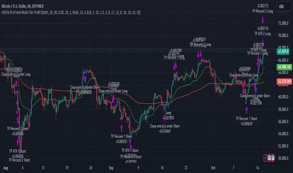
VIDYA ProTrend Multi-Tier ProfitHello! This time is about a trend-following system.
VIDYA is quite an interesting indicator that adjusts dynamically to market volatility, making it more responsive to price changes compared to traditional moving averages. Balancing adaptability and precision, especially with the more aggressive short trade settings, challenged me to fine-tune the strategy for a variety of market conditions.
█ Introduction and How it is Different
The "VIDYA ProTrend Multi-Tier Profit" strategy is a trend-following system that combines the VIDYA (Variable Index Dynamic Average) indicator with Bollinger Bands and a multi-step take-profit mechanism.
Unlike traditional trend strategies, this system allows for more adaptive profit-taking, adjusting for long and short positions through distinct ATR-based and percentage-based targets. The innovation lies in its dynamic multi-tier approach to profit-taking, especially for short trades, where more aggressive percentages are applied using a multiplier. This flexibility helps adapt to various market conditions by optimizing trade management and profit allocation based on market volatility and trend strength.
BTCUSD 6hr performance
█ Strategy, How it Works: Detailed Explanation
The core of the "VIDYA ProTrend Multi-Tier Profit" strategy lies in the dual VIDYA indicators (fast and slow) that analyze price trends while accounting for market volatility. These indicators work alongside Bollinger Bands to filter trade entries and exits.
🔶 VIDYA Calculation
The VIDYA indicator is calculated using the following formula:
Smoothing factor (𝛼):
alpha = 2 / (Length + 1)
VIDYA formula:
VIDYA(t) = alpha * k * Price(t) + (1 - alpha * k) * VIDYA(t-1)
Where:
k = |Chande Momentum Oscillator (MO)| / 100
🔶 Bollinger Bands as a Volatility Filter
Bollinger Bands are calculated using a rolling mean and standard deviation of price over a specified period:
Upper Band:
BB_upper = MA + (K * stddev)
Lower Band:
BB_lower = MA - (K * stddev)
Where:
MA is the moving average,
K is the multiplier (typically 2), and
stddev is the standard deviation of price over the Bollinger Bands length.
These bands serve as volatility filters to identify potential overbought or oversold conditions, aiding in the entry and exit logic.
🔶 Slope Calculation for VIDYA
The slopes of both fast and slow VIDYAs are computed to assess the momentum and direction of the trend. The slope for a given VIDYA over its length is:
Slope = (VIDYA(t) - VIDYA(t-n)) / n
Where:
n is the length of the lookback period. Positive slope indicates bullish momentum, while negative slope signals bearish momentum.
LOCAL picture
🔶 Entry and Exit Conditions
- Long Entry: Occurs when the price moves above the slow VIDYA and the fast VIDYA is trending upward. Bollinger Bands confirm the signal when the price crosses the upper band, indicating bullish strength.
- Short Entry: Happens when the price drops below the slow VIDYA and the fast VIDYA trends downward. The signal is confirmed when the price crosses the lower Bollinger Band, showing bearish momentum.
- Exit: Based on VIDYA slopes flattening or reversing, or when the price hits specific ATR or percentage-based profit targets.
🔶 Multi-Step Take Profit Mechanism
The strategy incorporates three levels of take profit for both long and short trades:
- ATR-based Take Profit: Each step applies a multiple of the ATR (Average True Range) to the entry price to define the exit point.
The first level of take profit (long):
TP_ATR1_long = Entry Price + (2.618 * ATR)
etc.
█ Trade Direction
The strategy offers flexibility in defining the trading direction:
- Long: Only long trades are considered based on the criteria for upward trends.
- Short: Only short trades are initiated in bearish trends.
- Both: The strategy can take both long and short trades depending on the market conditions.
█ Usage
To use the strategy effectively:
- Adjust the VIDYA lengths (fast and slow) based on your preference for trend sensitivity.
- Use Bollinger Bands as a filter for identifying potential breakout or reversal scenarios.
- Enable the multi-step take profit feature to manage positions dynamically, allowing for partial exits as the price reaches specified ATR or percentage levels.
- Leverage the short trade multiplier for more aggressive take profit levels in bearish markets.
This strategy can be applied to different asset classes, including equities, forex, and cryptocurrencies. Adjust the input parameters to suit the volatility and characteristics of the asset being traded.
█ Default Settings
The default settings for this strategy have been designed for moderate to trending markets:
- Fast VIDYA Length (10): A shorter length for quick responsiveness to price changes. Increasing this length will reduce noise but may delay signals.
- Slow VIDYA Length (30): The slow VIDYA is set longer to capture broader market trends. Shortening this value will make the system more reactive to smaller price swings.
- Minimum Slope Threshold (0.05): This threshold helps filter out weak trends. Lowering the threshold will result in more trades, while raising it will restrict trades to stronger trends.
Multi-Step Take Profit Settings
- ATR Multipliers (2.618, 5.0, 10.0): These values define how far the price should move before taking profit. Larger multipliers widen the profit-taking levels, aiming for larger trend moves. In higher volatility markets, these values might be adjusted downwards.
- Percentage Levels (3%, 8%, 17%): These percentage levels define how much the price must move before taking profit. Increasing the percentages will capture larger moves, while smaller percentages offer quicker exits.
- Short TP Multiplier (1.5): This multiplier applies more aggressive take profit levels for short trades. Adjust this value based on the aggressiveness of your short trade management.
Each of these settings directly impacts the performance and risk profile of the strategy. Shorter VIDYA lengths and lower slope thresholds will generate more trades but may result in more whipsaws. Higher ATR multipliers or percentage levels can delay profit-taking, aiming for larger trends but risking partial gains if the trend reverses too early.
Fibonacci & Bollinger Bands StrategyThis strategy combines Bollinger Bands and Fibonacci retracement/extension levels to identify potential entry and exit points in the market. Here’s a breakdown of each component and how the strategy works:
1. Bollinger Bands:
Bollinger Bands consist of a simple moving average (SMA) and two standard deviations (upper and lower bands) plotted above and below the SMA. The bands expand and contract based on market volatility.
Purpose in Strategy:
The lower band represents an area where the market might be oversold.
The upper band represents an area where the market might be overbought.
The price crossing these bands suggests overextended market conditions, which can be used to identify potential reversals.
2. Fibonacci Retracement and Extension Levels:
Fibonacci retracement levels are horizontal lines that indicate where price might find support or resistance as it retraces some of its previous movement. Common retracement levels are 61.8% and 78.6%.
Fibonacci extension levels are used to project areas where the price might extend after completing a retracement. These levels can help determine potential targets after a significant price movement.
Purpose in Strategy:
The strategy calculates the most recent swing high (fibHigh) and swing low (fibLow) over a lookback period. It then plots Fibonacci retracement and extension levels based on this range.
The Fibonacci levels are used as key support and resistance areas. The price approaching or touching these levels signals potential turning points in the market.
3. Entry Criteria:
A long position (buy) is triggered when:
The price crosses below the lower Bollinger Band, indicating an oversold condition.
The price is near or above a Fibonacci extension level (calculated based on the most recent price swing).
This suggests that the price is potentially reaching a strong support area, where a reversal is likely.
4. Exit Criteria:
The long position is closed (exit trade) when either:
The price touches or crosses the upper Bollinger Band, signaling an overbought condition.
The price reaches a Fibonacci retracement level or exceeds the recent swing high (fibHigh), indicating a potential exhaustion point or a reversal area.
5. General Strategy Logic:
The strategy takes advantage of market volatility (captured by the Bollinger Bands) and key support/resistance levels (determined by Fibonacci retracement and extension levels).
By combining these two techniques, the strategy identifies potential entry points at oversold levels with the expectation that the market will retrace or reverse upward, especially when near key Fibonacci extension levels.
Exit points are identified by potential overbought levels (Bollinger upper band) or key Fibonacci retracement levels, where the price might reverse downward.
6. Conditions to Execute the Strategy:
The Fibonacci levels are only calculated once the price has made a significant movement, establishing a recent high and low over a 50-bar period (which you can adjust). This ensures the Fibonacci levels are based on meaningful swings.
The entry and exit signals are filtered using both Bollinger Bands and Fibonacci levels to ensure that trades are not taken solely based on one indicator, thus reducing false signals.
Key Features of the Strategy:
Trend-following with reversal: It tries to catch reversals when the price hits extreme levels (Bollinger Bands) while respecting important Fibonacci levels.
Dynamic market adaptation: The strategy adapts to market conditions as it recalculates Fibonacci levels based on recent price swings and adjusts the Bollinger Bands for market volatility.
Confirmation through multiple indicators: It uses both the volatility-based signals from Bollinger Bands and the price structure from Fibonacci levels to confirm trade entries and exits.
Summary of the Strategy:
The strategy looks to buy low and sell high based on oversold/overbought signals from Bollinger Bands and Fibonacci levels that indicate key support and resistance zones.
By combining these two technical indicators, the strategy aims to reduce risk and increase accuracy by only entering trades when both indicators suggest favorable conditions.

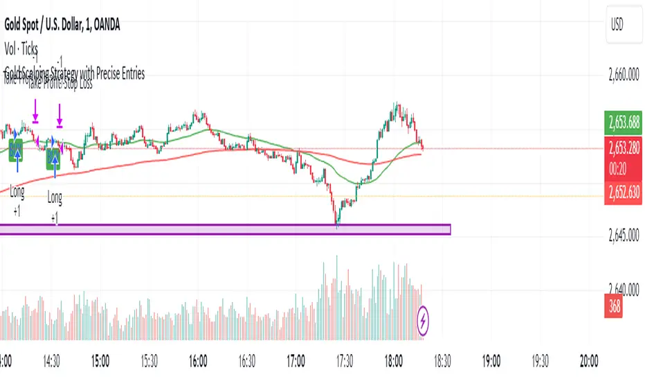
Gold Scalping Strategy with Precise EntriesThe Gold Scalping Strategy with Precise Entries is designed to take advantage of short-term price movements in the gold market (XAU/USD). This strategy uses a combination of technical indicators and chart patterns to identify precise buy and sell opportunities during times of consolidation and trend continuation.
Key Elements of the Strategy:
Exponential Moving Averages (EMAs):
50 EMA: Used as the shorter-term moving average to detect the recent price trend.
200 EMA: Used as the longer-term moving average to determine the overall market trend.
Trend Identification:
A bullish trend is identified when the 50 EMA is above the 200 EMA.
A bearish trend is identified when the 50 EMA is below the 200 EMA.
Average True Range (ATR):
ATR (14) is used to calculate the market's volatility and to set a dynamic stop loss based on recent price movements. Higher ATR values indicate higher volatility.
ATR helps define a suitable stop-loss distance from the entry point.
Relative Strength Index (RSI):
RSI (14) is used as a momentum oscillator to detect overbought or oversold conditions.
However, in this strategy, the RSI is primarily used as a consolidation filter to look for neutral zones (between 45 and 55), which may indicate a potential breakout or trend continuation after a consolidation phase.
Engulfing Patterns:
Bullish Engulfing: A bullish signal is generated when the current candle fully engulfs the previous bearish candle, indicating potential upward momentum.
Bearish Engulfing: A bearish signal is generated when the current candle fully engulfs the previous bullish candle, signaling potential downward momentum.
Precise Entry Conditions:
Long (Buy):
The 50 EMA is above the 200 EMA (bullish trend).
The RSI is between 45 and 55 (neutral/consolidation zone).
A bullish engulfing pattern occurs.
The price closes above the 50 EMA.
Short (Sell):
The 50 EMA is below the 200 EMA (bearish trend).
The RSI is between 45 and 55 (neutral/consolidation zone).
A bearish engulfing pattern occurs.
The price closes below the 50 EMA.
Take Profit and Stop Loss:
Take Profit: A fixed 20-pip target (where 1 pip = 0.10 movement in gold) is used for each trade.
Stop Loss: The stop-loss is dynamically set based on the ATR, ensuring that it adapts to current market volatility.
Visual Signals:
Buy and sell signals are visually plotted on the chart using green and red labels, indicating precise points of entry.
Advantages of This Strategy:
Trend Alignment: The strategy ensures that trades are taken in the direction of the overall trend, as indicated by the 50 and 200 EMAs.
Volatility Adaptation: The use of ATR allows the stop loss to adapt to the current market conditions, reducing the risk of premature exits in volatile markets.
Precise Entries: The combination of engulfing patterns and the neutral RSI zone provides a high-probability entry signal that captures momentum after consolidation.
Quick Scalping: With a fixed 20-pip profit target, the strategy is designed to capture small price movements quickly, which is ideal for scalping.
This strategy can be applied to lower timeframes (such as 1-minute, 5-minute, or 15-minute charts) for frequent trade opportunities in gold trading, making it suitable for day traders or scalpers. However, proper risk management should always be used due to the inherent volatility of gold.
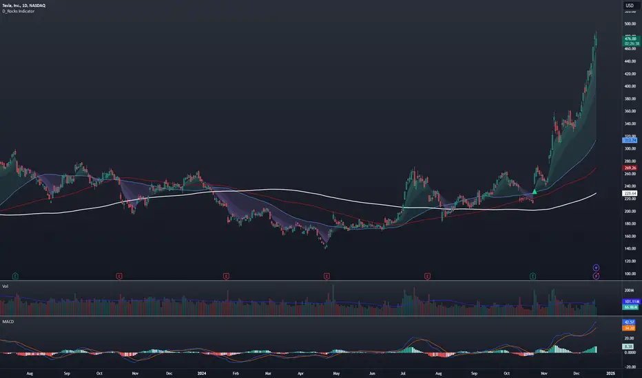
D_Rock's MA IndicatorD_Rock's Moving Average Indicator
This is an indicator version of my strategy linked here
**Overview:**
The basic concept of this indicator is to generate a signal when a faster/shorter length moving average crosses over (for Longs) or crosses under (for Shorts) a medium/longer length moving average. All of which are customizable. This indicator can work on any timeframe, however the daily is the timeframe used for the default settings and screenshots, as it was designed to be a multi-day swing strategy. Once a signal has been confirmed with a candle close, based on user options, the strategy is to enter the trade on the open of the next candle.
The crossover strategy is nothing new to trading, but what can make this strategy unique and helpful, is the addition of further confirmation points before a signal is generated along with the ability to show multiple moving averages on the chart if you choose. Each moving average pair can also be turned into a "cloud" instead of the traditional lines, for additional viewing preferences. Just about everything visual can be toggled on/off as well.
This indicator is a Trend (MA) indicator with optional confirmation points using a Momentum (MACD) indicator. While a Volume-based indicator is not shown here, one could consider using their favorite from that category to further compliment the signal idea.
If you would like to see the backtesting results for your favorite moving average crossover/under, please see my strategy version linked here .
Shoutout given to Ripster's Clouds Indicator as pieces of that code were taken and modified to create both the Cloud visualization effects, and the Moving Average Pair Plots that are implemented in this strategy.
MOVING AVERAGE OPTIONS
Select between and change the length & type of up to 5 pairs (10 total) of moving averages
The "Show Cloud-x" option will display a fill color between the "a" and "b" pairs
All moving averages lines can be toggled on/off in the "Style" tab, as well as adjusting their colors.
Visualization features do not affect calculations, meaning you could have all or nothing on the chart and the strategy will still produce results
SIGNAL CHOICES
Choose the fast/shorter length MA and the medium/longer length MA to determine the entry signal
CONFIRMATION OPTIONS
Both of these have customizable values and can be toggled on/off
A candle close over a slower/much longer length moving average
An additional cross-over (cross-under for Shorts) on the MACD indicator using default MACD values. While the MACD indicator is not necessary to have on the chart, it can help to add that for visualization. The calculations will perform whether the indicator is on the chart or not.
ADDITIONAL PLOTS
MACD (Moving Average Convergence/Divergence):
- The MACD is an optional confirmation indicator for this strategy.
- Plotting the indicator is not necessary for the strategy to work, but it can be helpful to visually see the status and position of the MACD if this feature is enabled in the strategy
- This helps to identify if there is also momentum behind the entry signal
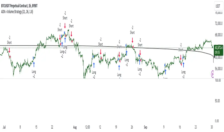
ADX + Volume Strategy### Strategy Description: ADX and Volume-Based Trading Strategy
This strategy is designed to identify strong market trends using the **Average Directional Index (ADX)** and confirm trading signals with **Volume**. The idea behind the strategy is to enter trades only when the market shows a strong trend (as indicated by ADX) and when the price movement is supported by high trading volume. This combination helps filter out weaker signals and provides more reliable entries into positions.
### Key Indicators:
1. **ADX (Average Directional Index)**:
- **Purpose**: ADX is a technical indicator that measures the strength of a trend, regardless of its direction (up or down).
- **Usage**: The strategy uses ADX to determine whether the market is trending strongly. If ADX is above a certain threshold (default is 25), it indicates that a strong trend is present.
- **Directional Indicators**:
- **DI+ (Directional Indicator Plus)**: Indicates the strength of the upward price movement.
- **DI- (Directional Indicator Minus)**: Indicates the strength of the downward price movement.
- ADX does not indicate the direction of the trend but confirms that a trend exists. DI+ and DI- are used to determine the direction.
2. **Volume**:
- **Purpose**: Volume is a key indicator for confirming the strength of a price movement. High volume suggests that a large number of market participants are supporting the movement, making it more likely to continue.
- **Usage**: The strategy compares the current volume to the 20-period moving average of the volume. The trade signal is confirmed if the current volume is greater than the average volume by a specified **Volume Multiplier** (default multiplier is 1.5). This ensures that the trade is supported by strong market participation.
### Strategy Logic:
#### **Entry Conditions:**
1. **Long Position** (Buy):
- **ADX** is above the threshold (default is 25), indicating a strong trend.
- **DI+ > DI-**, signaling that the market is trending upward.
- The **current volume** is greater than the 20-period average volume multiplied by the **Volume Multiplier** (e.g., 1.5), indicating that the upward price movement is backed by sufficient market activity.
2. **Short Position** (Sell):
- **ADX** is above the threshold (default is 25), indicating a strong trend.
- **DI- > DI+**, signaling that the market is trending downward.
- The **current volume** is greater than the 20-period average volume multiplied by the **Volume Multiplier** (e.g., 1.5), indicating that the downward price movement is backed by strong selling activity.
#### **Exit Conditions**:
- Positions are closed when the opposite signal appears:
- **For long positions**: Close when the short conditions are met (ADX still above the threshold, DI- > DI+, and the volume condition holds).
- **For short positions**: Close when the long conditions are met (ADX still above the threshold, DI+ > DI-, and the volume condition holds).
### Parameters:
- **ADX Period**: The period used to calculate ADX (default is 14). This controls how sensitive the ADX is to price movements.
- **ADX Threshold**: The minimum ADX value required for the strategy to consider the market trend as strong (default is 25). Higher values focus on stronger trends.
- **Volume Multiplier**: This parameter adjusts how much higher the current volume needs to be compared to the 20-period moving average for the signal to be valid. A value of 1.5 means the current volume must be 50% higher than the average volume.
### Example Trade Flow:
1. **Long Trade Example**:
- ADX > 25, confirming a strong trend.
- DI+ > DI-, confirming that the trend direction is upward.
- The current volume is 50% higher than the 20-period average volume (multiplied by 1.5).
- **Action**: Enter a long position.
2. **Short Trade Example**:
- ADX > 25, confirming a strong trend.
- DI- > DI+, confirming that the trend direction is downward.
- The current volume is 50% higher than the 20-period average volume.
- **Action**: Enter a short position.
### Strengths of the Strategy:
- **Trend Filtering**: The strategy ensures that trades are only taken when the market is trending strongly (confirmed by ADX) and that the price movement is supported by high volume, reducing the likelihood of false signals.
- **Volume Confirmation**: Using volume as confirmation provides an additional layer of reliability, as volume spikes often accompany sustained price moves.
- **Dual Signal Confirmation**: Both trend strength (ADX) and volume conditions must be met for a trade, making the strategy more robust.
### Weaknesses of the Strategy:
- **Limited Effectiveness in Range-Bound Markets**: Since the strategy relies on strong trends, it may underperform in sideways or non-trending markets where ADX stays below the threshold.
- **Lagging Nature of ADX**: ADX is a lagging indicator, which means that it may confirm the trend after it has already begun, potentially leading to late entries.
- **Volume Requirement**: In low-volume markets, the volume multiplier condition may not be met often, leading to fewer trade opportunities.
### Customization:
- **Adjust the ADX Threshold**: You can raise the threshold if you want to focus only on very strong trends, or lower it to capture moderate trends.
- **Adjust the Volume Multiplier**: You can change the multiplier to be more or less strict. A higher multiplier (e.g., 2.0) will require a stronger volume spike to confirm the signal, while a lower multiplier (e.g., 1.2) will allow more trades with weaker volume confirmation.
### Summary:
This ADX and Volume strategy is ideal for traders who want to follow strong trends while ensuring that the trend is supported by high trading volume. By combining a trend strength filter (ADX) and volume confirmation, the strategy aims to increase the probability of entering profitable trades while reducing the number of false signals. However, it may underperform in range-bound markets or in markets with low volume.
analytics_tablesLibrary "analytics_tables"
📝 Description
This library provides the implementation of several performance-related statistics and metrics, presented in the form of tables.
The metrics shown in the afforementioned tables where developed during the past years of my in-depth analalysis of various strategies in an atempt to reason about the performance of each strategy.
The visualization and some statistics where inspired by the existing implementations of the "Seasonality" script, and the performance matrix implementations of @QuantNomad and @ZenAndTheArtOfTrading scripts.
While this library is meant to be used by my strategy framework "Template Trailing Strategy (Backtester)" script, I wrapped it in a library hoping this can be usefull for other community strategy scripts that will be released in the future.
🤔 How to Guide
To use the functionality this library provides in your script you have to import it first!
Copy the import statement of the latest release by pressing the copy button below and then paste it into your script. Give a short name to this library so you can refer to it later on. The import statement should look like this:
import jason5480/analytics_tables/1 as ant
There are three types of tables provided by this library in the initial release. The stats table the metrics table and the seasonality table.
Each one shows different kinds of performance statistics.
The table UDT shall be initialized once using the `init()` method.
They can be updated using the `update()` method where the updated data UDT object shall be passed.
The data UDT can also initialized and get updated on demend depending on the use case
A code example for the StatsTable is the following:
var ant.StatsData statsData = ant.StatsData.new()
statsData.update(SideStats.new(), SideStats.new(), 0)
if (barstate.islastconfirmedhistory or (barstate.isrealtime and barstate.isconfirmed))
var statsTable = ant.StatsTable.new().init(ant.getTablePos('TOP', 'RIGHT'))
statsTable.update(statsData)
A code example for the MetricsTable is the following:
var ant.StatsData statsData = ant.StatsData.new()
statsData.update(ant.SideStats.new(), ant.SideStats.new(), 0)
if (barstate.islastconfirmedhistory or (barstate.isrealtime and barstate.isconfirmed))
var metricsTable = ant.MetricsTable.new().init(ant.getTablePos('BOTTOM', 'RIGHT'))
metricsTable.update(statsData, 10)
A code example for the SeasonalityTable is the following:
var ant.SeasonalData seasonalData = ant.SeasonalData.new().init(Seasonality.monthOfYear)
seasonalData.update()
if (barstate.islastconfirmedhistory or (barstate.isrealtime and barstate.isconfirmed))
var seasonalTable = ant.SeasonalTable.new().init(seasonalData, ant.getTablePos('BOTTOM', 'LEFT'))
seasonalTable.update(seasonalData)
🏋️♂️ Please refer to the "EXAMPLE" regions of the script for more advanced and up to date code examples!
Special thanks to @Mrcrbw for the proposal to develop this library and @DCNeu for the constructive feedback 🏆.
getTablePos(ypos, xpos)
Get table position compatible string
Parameters:
ypos (simple string) : The position on y axise
xpos (simple string) : The position on x axise
Returns: The position to be passed to the table
method init(this, pos, height, width, positiveTxtColor, negativeTxtColor, neutralTxtColor, positiveBgColor, negativeBgColor, neutralBgColor)
Initialize the stats table object with the given colors in the given position
Namespace types: StatsTable
Parameters:
this (StatsTable) : The stats table object
pos (simple string) : The table position string
height (simple float) : The height of the table as a percentage of the charts height. By default, 0 auto-adjusts the height based on the text inside the cells
width (simple float) : The width of the table as a percentage of the charts height. By default, 0 auto-adjusts the width based on the text inside the cells
positiveTxtColor (simple color) : The text color when positive
negativeTxtColor (simple color) : The text color when negative
neutralTxtColor (simple color) : The text color when neutral
positiveBgColor (simple color) : The background color with transparency when positive
negativeBgColor (simple color) : The background color with transparency when negative
neutralBgColor (simple color) : The background color with transparency when neutral
method init(this, pos, height, width, neutralBgColor)
Initialize the metrics table object with the given colors in the given position
Namespace types: MetricsTable
Parameters:
this (MetricsTable) : The metrics table object
pos (simple string) : The table position string
height (simple float) : The height of the table as a percentage of the charts height. By default, 0 auto-adjusts the height based on the text inside the cells
width (simple float) : The width of the table as a percentage of the charts width. By default, 0 auto-adjusts the width based on the text inside the cells
neutralBgColor (simple color) : The background color with transparency when neutral
method init(this, seas)
Initialize the seasonal data
Namespace types: SeasonalData
Parameters:
this (SeasonalData) : The seasonal data object
seas (simple Seasonality) : The seasonality of the matrix data
method init(this, data, pos, maxNumOfYears, height, width, extended, neutralTxtColor, neutralBgColor)
Initialize the seasonal table object with the given colors in the given position
Namespace types: SeasonalTable
Parameters:
this (SeasonalTable) : The seasonal table object
data (SeasonalData) : The seasonality data of the table
pos (simple string) : The table position string
maxNumOfYears (simple int) : The maximum number of years that fit into the table
height (simple float) : The height of the table as a percentage of the charts height. By default, 0 auto-adjusts the height based on the text inside the cells
width (simple float) : The width of the table as a percentage of the charts width. By default, 0 auto-adjusts the width based on the text inside the cells
extended (simple bool) : The seasonal table with extended columns for performance
neutralTxtColor (simple color) : The text color when neutral
neutralBgColor (simple color) : The background color with transparency when neutral
method update(this, wins, losses, numOfInconclusiveExits)
Update the strategy info data of the strategy
Namespace types: StatsData
Parameters:
this (StatsData) : The strategy statistics object
wins (SideStats)
losses (SideStats)
numOfInconclusiveExits (int) : The number of inconclusive trades
method update(this, stats, positiveTxtColor, negativeTxtColor, negativeBgColor, neutralBgColor)
Update the stats table object with the given data
Namespace types: StatsTable
Parameters:
this (StatsTable) : The stats table object
stats (StatsData) : The stats data to update the table
positiveTxtColor (simple color) : The text color when positive
negativeTxtColor (simple color) : The text color when negative
negativeBgColor (simple color) : The background color with transparency when negative
neutralBgColor (simple color) : The background color with transparency when neutral
method update(this, stats, buyAndHoldPerc, positiveTxtColor, negativeTxtColor, positiveBgColor, negativeBgColor)
Update the metrics table object with the given data
Namespace types: MetricsTable
Parameters:
this (MetricsTable) : The metrics table object
stats (StatsData) : The stats data to update the table
buyAndHoldPerc (float) : The buy and hold percetage
positiveTxtColor (simple color) : The text color when positive
negativeTxtColor (simple color) : The text color when negative
positiveBgColor (simple color) : The background color with transparency when positive
negativeBgColor (simple color) : The background color with transparency when negative
method update(this)
Update the seasonal data based on the season and eon timeframe
Namespace types: SeasonalData
Parameters:
this (SeasonalData) : The seasonal data object
method update(this, data, positiveTxtColor, negativeTxtColor, neutralTxtColor, positiveBgColor, negativeBgColor, neutralBgColor, timeBgColor)
Update the seasonal table object with the given data
Namespace types: SeasonalTable
Parameters:
this (SeasonalTable) : The seasonal table object
data (SeasonalData) : The seasonal cell data to update the table
positiveTxtColor (simple color) : The text color when positive
negativeTxtColor (simple color) : The text color when negative
neutralTxtColor (simple color) : The text color when neutral
positiveBgColor (simple color) : The background color with transparency when positive
negativeBgColor (simple color) : The background color with transparency when negative
neutralBgColor (simple color) : The background color with transparency when neutral
timeBgColor (simple color) : The background color of the time gradient
SideStats
Object that represents the strategy statistics data of one side win or lose
Fields:
numOf (series int)
sumFreeProfit (series float)
freeProfitStDev (series float)
sumProfit (series float)
profitStDev (series float)
sumGain (series float)
gainStDev (series float)
avgQuantityPerc (series float)
avgCapitalRiskPerc (series float)
avgTPExecutedCount (series float)
avgRiskRewardRatio (series float)
maxStreak (series int)
StatsTable
Object that represents the stats table
Fields:
table (series table) : The actual table
rows (series int) : The number of rows of the table
columns (series int) : The number of columns of the table
StatsData
Object that represents the statistics data of the strategy
Fields:
wins (SideStats)
losses (SideStats)
numOfInconclusiveExits (series int)
avgFreeProfitStr (series string)
freeProfitStDevStr (series string)
lossFreeProfitStDevStr (series string)
avgProfitStr (series string)
profitStDevStr (series string)
lossProfitStDevStr (series string)
avgQuantityStr (series string)
MetricsTable
Object that represents the metrics table
Fields:
table (series table) : The actual table
rows (series int) : The number of rows of the table
columns (series int) : The number of columns of the table
SeasonalData
Object that represents the seasonal table dynamic data
Fields:
seasonality (series Seasonality)
eonToMatrixRow (map)
numOfEons (series int)
mostRecentMatrixRow (series int)
balances (matrix)
returnPercs (matrix)
maxDDs (matrix)
eonReturnPercs (array)
eonCAGRs (array)
eonMaxDDs (array)
SeasonalTable
Object that represents the seasonal table
Fields:
table (series table) : The actual table
headRows (series int) : The number of head rows of the table
headColumns (series int) : The number of head columns of the table
eonRows (series int) : The number of eon rows of the table
seasonColumns (series int) : The number of season columns of the table
statsRows (series int)
statsColumns (series int) : The number of stats columns of the table
rows (series int) : The number of rows of the table
columns (series int) : The number of columns of the table
extended (series bool) : Whether the table has additional performance statistics

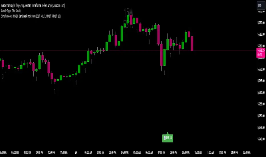
Simultaneous INSIDE Bar Break IndicatorSimultaneous Inside Bar Break Indicator (SIBBI) for The Strat Community
Overview:
The Simultaneous Inside Bar Break Indicator (SIBBI) is designed to help traders using The Strat methodology identify one of the most powerful breakout patterns: the Simultaneous Inside Bar Break across multiple symbols. This indicator detects when all four user-selected symbols form inside bars on the previous candle and then break those inside bars in the same direction (either bullish or bearish) on the current candle.
Inside bars represent consolidation periods where price action does not break the high or low of the previous candle. When a simultaneous break occurs across multiple symbols, this often signals a strong move in the market, making this a key actionable signal in The Strat trading strategy.
Key Features:
Multi-Symbol Analysis: You can track up to four different symbols simultaneously. By default, the indicator comes with SPY, QQQ, IWM, and DIA, but you can modify these to track any other assets or symbols.
Inside Bar Detection: The indicator checks whether all four symbols have inside bars on the previous candle. It only triggers when all symbols meet this condition, making it a highly specific and reliable signal.
Simultaneous Break Detection: Once all symbols have inside bars, the indicator waits for a breakout in the same direction across all four symbols. A simultaneous bullish break (prices breaking above the previous candle’s high) triggers a green label, while a simultaneous bearish break (prices breaking below the previous candle’s low) triggers a red label.
Dynamic Label Timeframe: The indicator dynamically adjusts the timeframe in the label based on the user’s selected timeframe. This allows traders to know precisely which timeframe the break is occurring on. If the user selects "Chart Timeframe," the indicator will evolve with the current chart's timeframe, making it more versatile.
Timeframe Flexibility: The indicator can be set to analyze any timeframe—15-minute, 30-minute, 60-minute, daily, weekly, and so on. It only works for the specific timeframe you set it to in the settings. If set to "Chart Timeframe," the label will adapt dynamically based on the timeframe you are currently viewing.
Customizable Labels: The user can choose the size of the labels (tiny, small, or normal), ensuring that the visual output is tailored to individual preferences and chart layouts.
Best Use Case:
The Simultaneous Inside Bar Break Indicator is particularly powerful when applied to multiple timeframes. Here’s how to use it for maximum impact:
Multi-Timeframe Setup: Set the indicator on various timeframes (e.g., 15-minute, 30-minute, 60-minute, and daily) across multiple charts. This allows you to monitor different timeframes and identify when lower timeframe breaks trigger potential moves on higher timeframes.
Anticipating Strong Moves: When a simultaneous inside bar break occurs on one timeframe (e.g., 30-minute), keep an eye on the higher timeframes (e.g., 60-minute or daily) to see if those timeframes also break. This stacking of inside bar breaks can signal powerful market moves.
Higher Conviction Signals: The indicator is designed to provide high-conviction signals. Since it requires all four symbols to break in the same direction simultaneously, it reduces false signals and focuses on higher probability setups, which is crucial for traders using The Strat to time their trades effectively.
How the Indicator Works:
Inside Bar Formation: The indicator first checks that all four selected symbols had inside bars in the previous bar (i.e., the current high and low are contained within the previous bar’s high and low).
Simultaneous Break Detection: After detecting inside bars, the indicator checks if all four symbols break out in the same direction—bullish (breaking above the previous bar’s high) or bearish (breaking below the previous bar’s low).
Label Display: When a simultaneous inside bar break occurs, a label is plotted on the chart—either green for a bullish break (below the candle) or red for a bearish break (above the candle). The label will display the timeframe you set in the settings (e.g., "IBSB 60" for a 60-minute break).
Chart Timeframe Option: If you prefer, you can set the indicator to evolve with the chart’s current timeframe. In this mode, the label will not show a specific timeframe but will still display the simultaneous inside bar break when it occurs.
Recommendations for Usage:
Focus on Multiple Timeframes: The Strat methodology is all about understanding the relationship between different timeframes. Use this indicator on multiple timeframes to get a better picture of potential moves.
Pair with Other Strat Techniques: This indicator is most powerful when combined with other Strat tools, such as broadening formations, timeframe continuity, and actionable signals (e.g., 2-2 reversals). The simultaneous inside bar break can help confirm or invalidate other signals.
Customize Symbols and Timeframes: Although the default symbols are SPY, QQQ, IWM, and DIA, feel free to replace them with symbols more relevant to your trading. This indicator works well across equities, indices, futures, and forex pairs.
How to Set It Up:
Select Symbols: Choose four symbols that you want to track. These can be index ETFs (like SPY and QQQ), individual stocks, or any other tradable instruments.
Set Timeframe: In the indicator’s settings, choose a specific timeframe (e.g., 15-minute, 30-minute, daily). The label will reflect the selected timeframe, making it clear which time-based break you are seeing.
Optional - Chart Timeframe Mode: If you want the indicator to adapt to the chart’s current timeframe, select the "Chart Timeframe" option in the settings. The indicator will plot the breaks without showing a specific timeframe in the label.
Customize Label Size: Depending on your chart layout and personal preference, you can adjust the size of the labels (tiny, small, or normal) in the settings.
Conclusion:
The Simultaneous Inside Bar Break Indicator is a powerful tool for traders using The Strat methodology, offering a highly specific and reliable signal that can indicate potential large market moves. By monitoring multiple symbols and timeframes, you can gain deeper insight into the market's behavior and act with greater confidence. This indicator is ideal for traders looking to catch high-conviction moves and align their trades with broader market continuity.
Note: The indicator works best when paired with multi-timeframe analysis, allowing you to see how breaks on lower timeframes might influence larger trends. For traders who prefer simplicity, setting it to the "Chart Timeframe" mode offers flexibility while maintaining the core benefits of this indicator.
Multi-Step FlexiSuperTrend - Indicator [presentTrading]This version of the indicator is built upon the foundation of a strategy version published earlier. However, this indicator version focuses on providing visual insights and alerts for traders, rather than executing trades. This one is mostly for @thorcmt.
█ Introduction and How it is Different
The **Multi-Step FlexiSuperTrend Indicator** is a versatile tool designed to provide traders with a highly customizable and flexible approach to trend analysis. Unlike traditional supertrend indicators, which focus on a single factor or threshold, the **FlexiSuperTrend** allows users to define multiple levels of take-profit targets and incorporate different trend normalization methods.
It comes with several advanced customization features, including multi-step take profits, deviation plotting, and trend normalization, making it suitable for both novice and expert traders.
BTCUSD 6hr Performance
█ Strategy, How It Works: Detailed Explanation
The **Multi-Step FlexiSuperTrend** works by calculating a supertrend based on multiple factors and incorporating oscillations from trend deviations. Here’s a breakdown of how it functions:
🔶 SuperTrend Calculation
At the heart of the indicator is the SuperTrend formula, which dynamically adjusts based on price movements.
🔶 Normalization of Deviations
To enhance accuracy, the **FlexiSuperTrend** calculates multiple deviations from the trend and normalizes them.
🔶 Multi-Step Take Profit Levels
The indicator allows setting up to three take profit levels, which are displayed via price level alerts. lows traders to exit part of their position at various profit intervals.
For more detail, please check the strategy version - Multi-Step-FlexiSuperTrend-Strategy:
and 'FlexiSuperTrend-Strategy'
█ Trade Direction
The **Multi-Step FlexiSuperTrend Indicator** supports both long and short trade directions.
This flexibility allows traders to adapt to trending, volatile, or sideways markets.
█ Usage
To use the **FlexiSuperTrend Indicator**, traders can set up their preferences for the following key features:
- **Trading Direction**: Choose whether to focus on long, short, or both signals.
- **Indicator Source**: The price source to calculate the trend (e.g., close, hl2).
- **Indicator Length**: The number of periods to calculate the ATR and trend (the larger the value, the smoother the trend).
- **Starting and Increment Factor**: These adjust how reactive the trend is to price movements. The starting factor dictates how far the initial trend band is from the price, and the increment factor adjusts subsequent trend deviations.
The indicator then displays buy and sell signals on the chart, along with alerts for each take-profit level.
Local picture
█ Default Settings
The default settings of the **Multi-Step FlexiSuperTrend** are carefully designed to provide an optimal balance between sensitivity and accuracy. Let’s examine these default parameters and their effect on performance:
🔶 Indicator Length (Default: 10)
The **Indicator Length** determines the lookback period for the ATR calculation. A smaller value makes the indicator more reactive to price changes, but may generate more false signals. A longer length smooths the trend and reduces noise but may delay signals.
Effect on performance: Shorter lengths perform better in volatile markets, while longer lengths excel in trending markets.
🔶 Starting Factor (Default: 0.618)
This factor adjusts the starting distance of the SuperTrend from the current price. The smaller the starting factor, the closer the trend is to the price, making it more sensitive. Conversely, a larger factor allows more distance, reducing sensitivity but filtering out false signals.
Effect on performance: A smaller factor provides quicker signals but can lead to frequent false positives. A larger factor generates fewer but more reliable signals.
🔶 Increment Factor (Default: 0.382)
The **Increment Factor** controls how the trend bands adjust as the price moves. It increases the distance of the bands from the price with each iteration.
Effect on performance: A higher increment factor can result in wider stop-loss or trend reversal bands, allowing for longer trends to develop without frequent exits. A lower factor keeps the bands closer to the price and is more suited for shorter-term trades.
🔶 Take Profit Levels (Default: 2%, 8%, 18%)
The default take-profit levels are set at 2%, 8%, and 18%. These values represent the thresholds at which the trader can partially exit their positions. These multi-step levels are highly customizable depending on the trader’s risk tolerance and strategy.
Effect on performance: Lower take-profit levels (e.g., 2%) capture small, quick profits in volatile markets, while higher levels (8%-18%) allow for a more gradual exit in strong trends.
🔶 Normalization Method (Default: None)
The default normalization method is **None**, meaning the deviations are not normalized. However, enabling normalization (e.g., **Max-Min**) can improve the clarity of the indicator’s signals in volatile or choppy markets by smoothing out the noise.
Effect on performance: Using a normalization method can reduce the effect of extreme deviations, making signals more stable and less prone to false positives.

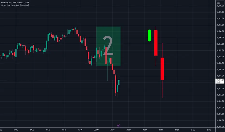
Higher Time Frame Strat [QuantVue]The Higher Time Frame Strat Indicator is a tool that helps traders visualize and analyze price action from a higher timeframe (HTF) on their current chart. It applies the Strat method, a trading strategy focused on identifying key price action setups by observing how current price bars relate to previous ones. This helps in understanding the market's structure and determining potential trading opportunities based on higher timeframe data.
Key Concepts:
Strat Basics:
Type 1 Bar (Inside Bar): The current bar's high is lower than the previous bar's high, and its low is higher than the previous bar's low. This signifies a consolidation, or indecision, as the price is contained within the previous bar's range.
Type 2 Bar (Directional Bar): The current bar either breaks above the previous bar's high (bullish) or stays above the previous bar's low (bearish), indicating a continuation in the price direction.
Type 3 Bar (Outside Bar): The current bar breaks both above the previous bar's high and below the previous bar's low, showing volatility and a potential reversal.
Higher Timeframe Visualization:
The indicator uses a user-defined higher timeframe (default: 1 hour) and plots the last three higher timeframe candles on the current chart.
Strat Classification:
When a new higher timeframe candle forms, the indicator draws a semi-transparent box around the candle's range (high to low), along with the Strat type label. This provides a visual cue to the trader about the structure of the newly formed candle and how it fits into the overall market movement.
The script classifies each higher timeframe candle as one of the Strat types (1, 2, or 3). Based on the relationship between the current candle and the previous candle's high/low, it assigns a label ("1", "2", or "3"), helping traders quickly identify the price action setup on the higher timeframe.
How to Use the Indicator:
Trend Continuation: Look for Type 2 bars, which indicate a continuation in the current trend. For example, a Type 2 up suggests the price is breaking above the previous high, potentially signaling further upward movement.
Reversals: Type 3 bars show increased volatility, where the price breaks both above and below the previous bar's range. This could indicate a reversal, so be prepared for a potential change in direction.
Consolidation: Inside bars (Type 1) signify a tightening range and can signal the beginning of a breakout once the price moves outside of the previous bar's high or low.
By combining these price action concepts with the visualization of higher timeframe data, traders can potentially get earlier entry and exits as a higher timeframe set up forms.
Post-Open Long Strategy with ATR-based Stop Loss and Take ProfitThe "Post-Open Long Strategy with ATR-Based Stop Loss and Take Profit" is designed to identify buying opportunities after the German and US markets open. It combines various technical indicators to filter entry signals, focusing on breakout moments following price lateralization periods.
Key Components and Their Interaction:
Bollinger Bands (BB):
Description: Uses BB with a 14-period length and standard deviation multiplier of 1.5, creating narrower bands for lower timeframes.
Role in the Strategy: Identifies low volatility phases (lateralization). The lateralization condition is met when the price is near the simple moving average of the BB, suggesting an imminent increase in volatility.
Exponential Moving Averages (EMA):
10-period EMA: Quickly detects short-term trend direction.
200-period EMA: Filters long-term trends, ensuring entries occur in a bullish market.
Interaction: Positions are entered only if the price is above both EMAs, indicating a consolidated positive trend.
Relative Strength Index (RSI):
Description: 7-period RSI with a threshold above 30.
Role in the Strategy: Confirms the market is not oversold, supporting the validity of the buy signal.
Average Directional Index (ADX):
Description: 7-period ADX with 7-period smoothing and a threshold above 10.
Role in the Strategy: Assesses trend strength. An ADX above 10 indicates sufficient momentum to justify entry.
Average True Range (ATR) for Dynamic Stop Loss and Take Profit:
Description: 14-period ATR with multipliers of 2.0 for Stop Loss and 4.0 for Take Profit.
Role in the Strategy: Adjusts exit levels based on current volatility, enhancing risk management.
Resistance Identification and Breakout:
Description: Analyzes the highs of the last 20 candles to identify resistance levels with at least two touches.
Role in the Strategy: A breakout above this level signals a potential continuation of the bullish trend.
Time Filters and Market Conditions:
Trading Hours: Operates only during the opening of the German market (8:00 - 12:00) and US market (15:30 - 19:00).
Panic Candle: The current candle must close negative, leveraging potential emotional reactions in the market.
Avoiding Entry During Pullbacks:
Description: Checks that the two previous candles are not both bearish.
Role in the Strategy: Avoids entering during a potential pullback, improving trade success probability.
Post-Open Long Strategy with ATR-Based Stop Loss and Take Profit
The "Post-Open Long Strategy with ATR-Based Stop Loss and Take Profit" is designed to identify buying opportunities after the German and US markets open. It combines various technical indicators to filter entry signals, focusing on breakout moments following price lateralization periods.
Key Components and Their Interaction:
Bollinger Bands (BB):
Description: Uses BB with a 14-period length and standard deviation multiplier of 1.5, creating narrower bands for lower timeframes.
Role in the Strategy: Identifies low volatility phases (lateralization). The lateralization condition is met when the price is near the simple moving average of the BB, suggesting an imminent increase in volatility.
Exponential Moving Averages (EMA):
10-period EMA: Quickly detects short-term trend direction.
200-period EMA: Filters long-term trends, ensuring entries occur in a bullish market.
Interaction: Positions are entered only if the price is above both EMAs, indicating a consolidated positive trend.
Relative Strength Index (RSI):
Description: 7-period RSI with a threshold above 30.
Role in the Strategy: Confirms the market is not oversold, supporting the validity of the buy signal.
Average Directional Index (ADX):
Description: 7-period ADX with 7-period smoothing and a threshold above 10.
Role in the Strategy: Assesses trend strength. An ADX above 10 indicates sufficient momentum to justify entry.
Average True Range (ATR) for Dynamic Stop Loss and Take Profit:
Description: 14-period ATR with multipliers of 2.0 for Stop Loss and 4.0 for Take Profit.
Role in the Strategy: Adjusts exit levels based on current volatility, enhancing risk management.
Resistance Identification and Breakout:
Description: Analyzes the highs of the last 20 candles to identify resistance levels with at least two touches.
Role in the Strategy: A breakout above this level signals a potential continuation of the bullish trend.
Time Filters and Market Conditions:
Trading Hours: Operates only during the opening of the German market (8:00 - 12:00) and US market (15:30 - 19:00).
Panic Candle: The current candle must close negative, leveraging potential emotional reactions in the market.
Avoiding Entry During Pullbacks:
Description: Checks that the two previous candles are not both bearish.
Role in the Strategy: Avoids entering during a potential pullback, improving trade success probability.
Entry and Exit Conditions:
Long Entry:
The price breaks above the identified resistance.
The market is in a lateralization phase with low volatility.
The price is above the 10 and 200-period EMAs.
RSI is above 30, and ADX is above 10.
No short-term downtrend is detected.
The last two candles are not both bearish.
The current candle is a "panic candle" (negative close).
Order Execution: The order is executed at the close of the candle that meets all conditions.
Exit from Position:
Dynamic Stop Loss: Set at 2 times the ATR below the entry price.
Dynamic Take Profit: Set at 4 times the ATR above the entry price.
The position is automatically closed upon reaching the Stop Loss or Take Profit.
How to Use the Strategy:
Application on Volatile Instruments:
Ideal for financial instruments that show significant volatility during the target market opening hours, such as indices or major forex pairs.
Recommended Timeframes:
Intraday timeframes, such as 5 or 15 minutes, to capture significant post-open moves.
Parameter Customization:
The default parameters are optimized but can be adjusted based on individual preferences and the instrument analyzed.
Backtesting and Optimization:
Backtesting is recommended to evaluate performance and make adjustments if necessary.
Risk Management:
Ensure position sizing respects risk management rules, avoiding risking more than 1-2% of capital per trade.
Originality and Benefits of the Strategy:
Unique Combination of Indicators: Integrates various technical metrics to filter signals, reducing false positives.
Volatility Adaptability: The use of ATR for Stop Loss and Take Profit allows the strategy to adapt to real-time market conditions.
Focus on Post-Lateralization Breakout: Aims to capitalize on significant moves following consolidation periods, often associated with strong directional trends.
Important Notes:
Commissions and Slippage: Include commissions and slippage in settings for more realistic simulations.
Capital Size: Use a realistic trading capital for the average user.
Number of Trades: Ensure backtesting covers a sufficient number of trades to validate the strategy (ideally more than 100 trades).
Warning: Past results do not guarantee future performance. The strategy should be used as part of a comprehensive trading approach.
With this strategy, traders can identify and exploit specific market opportunities supported by a robust set of technical indicators and filters, potentially enhancing their trading decisions during key times of the day.
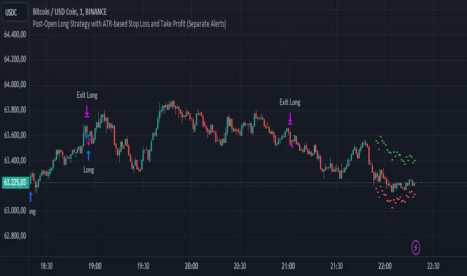
Trend Magic with EMA, SMA, and Auto-TradingRelease Notes
Strategy Name: Trend Magic with EMA, SMA, and Auto-Trading
Purpose: This strategy is designed to capture entry and exit points in the market using the Trend Magic indicator and three moving averages (EMA45, SMA90, and SMA180). Specifically, it uses the perfect order of the moving averages and the color changes in Trend Magic to identify trend reversals and potential trading opportunities.
Uniqueness and Usefulness
Uniqueness: The strategy utilizes the Trend Magic indicator, which is based on price and volatility, along with three moving averages to assess the strength of trends. The signals are generated only when the moving averages are in perfect order, and the Trend Magic color changes, ensuring that the entry is made during established trends. This combination provides a higher degree of reliability compared to strategies that rely solely on price action or single indicators.
Usefulness: This strategy is particularly useful for traders looking to capture trends over longer periods. It is effective at reducing noise in the market, only providing signals when the moving averages align and the Trend Magic indicator confirms a trend reversal. It works well in both trending and volatile markets.
Entry Conditions
Long Entry:
Condition: A perfect order (EMA45 > SMA90 > SMA180) is established, and Trend Magic changes color from red to blue.
Signal: A buy signal is generated, indicating the start of an uptrend.
Short Entry:
Condition: A perfect order (EMA45 < SMA90 < SMA180) is established, and Trend Magic changes color from blue to red.
Signal: A sell signal is generated, indicating the start of a downtrend.
Exit Conditions
Exit Strategy:
This strategy automatically enters and exits trades based on signals, but traders are encouraged to manage exits manually according to their own risk management preferences. The strategy includes stop loss and take profit settings based on risk-to-reward ratios for better risk management.
Risk Management
The strategy includes built-in risk management by using the SMA90 level at the time of entry as the stop-loss point and setting the take profit at a 1:1.5 risk-to-reward ratio. The stop-loss level is fixed at the entry point and does not move as the market progresses. Traders are advised to implement additional risk management, such as trailing stops, for added protection.
Account Size: ¥100,000
Commissions and Slippage: Assumes 94 pips for commissions and 1 pip for slippage per trade
Risk per Trade: 10% of account equity (adjust this based on personal risk tolerance)
Configurable Options
Configurable Options:
CCI Period: Set the period for the CCI used to calculate the Trend Magic indicator (default is 21).
ATR Multiplier: Set the multiplier for ATR used in the Trend Magic calculation (default is 1.0).
EMA/SMA Periods: The periods for the three moving averages (default is EMA45, SMA90, and SMA180).
Signal Display Control: An option to toggle the display of buy and sell signals on the chart.
Adequate Sample Size
To ensure the robustness and reliability of this strategy, it is recommended to backtest it with a sufficiently long period of historical data. Testing across different market conditions, including high and low volatility periods, is also advised.
Credits
Acknowledgments:
This strategy is based on the Trend Magic indicator combined with moving averages and draws on contributions from the technical analysis and trading community.
Clean Chart Description
Chart Appearance:
To maintain a clean and simple chart, this strategy includes options to turn off the display of Trend Magic, moving averages, and entry signals. Traders can adjust these display settings as needed to minimize visual clutter and focus on effective trend analysis.
Addressing the House Rule Violations
Omissions and Unrealistic Claims
Clarification:
This strategy does not make any unrealistic or unsupported claims about its performance. All signals are intended for educational purposes only and do not guarantee future results. It is important to note that past performance does not guarantee future outcomes, and proper risk management is crucial.

Sygnały Long/Short z SL i TPChoosing the Best Timeframe for Your Trading Strategy
The ideal timeframe for your trading strategy depends on several factors, including your trading style, risk preferences, and the goals of your strategy. Here’s a guide to different timeframes and their applications:
Timeframes and Their Uses:
Short-Term Timeframes (e.g., 5-minute, 15-minute):
Advantages: Provide more frequent signals and allow for quick responses to market changes. Ideal for day traders who prefer short, rapid trades.
Disadvantages: Can generate more false signals and be more susceptible to market noise. Requires more frequent attention and monitoring.
Medium-Term Timeframes (e.g., 1-hour, 4-hour):
Advantages: Offer fewer false signals compared to shorter timeframes. Suitable for swing traders looking to capture short-term trends.
Disadvantages: Fewer signals compared to shorter timeframes. Requires less frequent monitoring.
Long-Term Timeframes (e.g., daily, weekly):
Advantages: Provide more stable signals and are less affected by market noise. Ideal for long-term investors and those trading based on trends.
Disadvantages: Fewer signals, which may be less frequent but more reliable. Requires longer confirmation times.
Recommendation for Your Strategy:
For a strategy based on moving averages (MA) and generating long/short signals, the 5-minute and 15-minute timeframes might be suitable if:
You are a day trader and want to generate multiple signals per day.
You prefer quick responses to price changes and want to execute trades within a shorter timeframe.
For more stable signals and fewer false signals:
1-hour or 4-hour timeframes might be more appropriate.
Testing and Optimization:
Test Different Timeframes: See how your strategy performs on various timeframes to find the one that works best for you.
Adjust Parameters: Modify the lengths of the short and long SMAs, as well as the SL and TP levels, to fit the chosen timeframe.
How to Test:
Add the script to your chart on different timeframes on TradingView.
Observe the effectiveness and accuracy of the signals.
Adjust settings based on results and personal preferences.
Summary:
There isn’t a single “best” timeframe as it depends on your trading style and objectives. Start by testing on shorter timeframes if you are interested in day trading, and then explore how the strategy performs on longer timeframes for more stable signals.
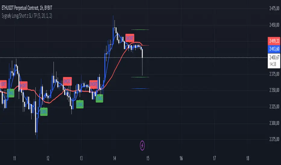
Larry Connors %b Strategy (Bollinger Band)Larry Connors’ %b Strategy is a mean-reversion trading approach that uses Bollinger Bands to identify buy and sell signals based on the %b indicator. This strategy was developed by Larry Connors, a renowned trader and author known for his systematic, data-driven trading methods, particularly those focusing on short-term mean reversion.
The %b indicator measures the position of the current price relative to the Bollinger Bands, which are volatility bands placed above and below a moving average. The strategy specifically targets times when prices are oversold within a long-term uptrend and aims to capture rebounds by buying at relatively low points and selling at relatively high points.
Strategy Rules
The basic rules of the %b Strategy are:
1. Trend Confirmation: The closing price must be above the 200-day moving average. This filter ensures that trades are made in alignment with a longer-term uptrend, thereby avoiding trades against the primary market trend.
2. Oversold Conditions: The %b indicator must be below 0.2 for three consecutive days. The %b value below 0.2 indicates that the price is near the lower Bollinger Band, suggesting an oversold condition.
3. Entry Signal: Enter a long position at the close when conditions 1 and 2 are met.
4. Exit Signal: Exit the position when the %b value closes above 0.8, signaling an overbought condition where the price is near the upper Bollinger Band.
How the Strategy Works
This strategy operates on the premise of mean reversion, which suggests that extreme price movements will revert to the mean over time. By entering positions when the %b value indicates an oversold condition (below 0.2) in a confirmed uptrend, the strategy attempts to capture short-term price rebounds. The exit rule (when %b is above 0.8) aims to lock in profits once the price reaches an overbought condition, often near the upper Bollinger Band.
Who Was Larry Connors?
Larry Connors is a well-known figure in the world of financial markets and trading. He co-authored several influential trading books, including “Short-Term Trading Strategies That Work” and “High Probability ETF Trading.” Connors is recognized for his quantitative approach, focusing on systematic, rules-based strategies that leverage historical data to validate trading edges.
His work primarily revolves around short-term trading strategies, often using technical indicators like RSI (Relative Strength Index), Bollinger Bands, and moving averages. Connors’ methodologies have been widely adopted by traders seeking structured approaches to exploit short-term inefficiencies in the market.
Risks of the Strategy
While the %b Strategy can be effective, particularly in mean-reverting markets, it is not without risks:
1. Mean Reversion Assumption: The strategy is based on the assumption that prices will revert to the mean. In trending or sharply falling markets, this reversion may not occur, leading to sustained losses.
2. False Signals in Choppy Markets: In volatile or sideways markets, the strategy may generate multiple false signals, resulting in whipsaw trades that can erode capital through frequent small losses.
3. No Stop Loss: The basic implementation of the strategy does not include a stop loss, which increases the risk of holding losing trades longer than intended, especially if the market continues to move against the position.
4. Performance During Market Crashes: During major market downturns, the strategy’s buy signals could be triggered frequently as prices decline, compounding losses without the presence of a risk management mechanism.
Scientific References and Theoretical Basis
The %b Strategy relies on the concept of mean reversion, which has been extensively studied in finance literature. Studies by Avellaneda and Lee (2010) and Bouchaud et al. (2018) have demonstrated that mean-reverting strategies can be profitable in specific market environments, particularly when combined with volatility filters like Bollinger Bands. However, the same studies caution that such strategies are highly sensitive to market conditions and often perform poorly during periods of prolonged trends.
Bollinger Bands themselves were popularized by John Bollinger and are widely used to assess price volatility and detect potential overbought and oversold conditions. The %b value is a critical part of this analysis, as it standardizes the position of price relative to the bands, making it easier to compare conditions across different securities and time frames.
Conclusion
Larry Connors’ %b Strategy is a well-known mean-reversion technique that leverages Bollinger Bands to identify buying opportunities in uptrending markets when prices are temporarily oversold. While the strategy can be effective under the right conditions, traders should be aware of its limitations and risks, particularly in trending or highly volatile markets. Incorporating risk management techniques, such as stop losses, could help mitigate some of these risks, making the strategy more robust against adverse market conditions.
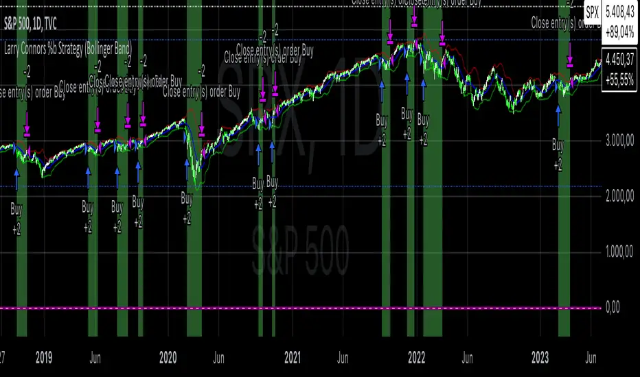
TRIN (Arms Index) Trading StrategyThe TRIN (Arms Index), also known as the Short-Term Trading Index, is a technical indicator designed to gauge the internal strength or weakness of the market. It compares the number of advancing and declining stocks to the advancing and declining volume (AD Volume). A TRIN value above 1.0 generally indicates bearish market conditions, while a value below 1.0 suggests bullish market sentiment.
Strategy Rules:
Entry Condition (Long Position): When the TRIN value is above 1.0, the strategy enters a long position, indicating that the market may be oversold, and a potential reversal could occur.
Exit Condition: The strategy exits the long position when the closing price is higher than the previous day’s high, signaling a potential rebound in the market.
This strategy aims to capitalize on short-term market inefficiencies by entering trades during periods of potential market weakness and exiting when signs of recovery appear.
How the TRIN Index Works:
The TRIN is calculated as follows:
TRIN=Advancing Issues / Declining IssuesAdvancing Volume / Declining Volume
TRIN=Advancing Volume / Declining VolumeAdvancing Issues / Declining Issues
A TRIN value above 1.0 indicates that the market is potentially oversold (more declining stocks with higher volume), while a value below 1.0 suggests the market may be overbought (more advancing stocks with higher volume) .
Empirical Evidence:
Market Sentiment Indicator: The TRIN has been widely used as a sentiment indicator. Research by Zweig (1997) suggests that extreme TRIN values can serve as a contrarian signal, indicating potential turning points in the market. For instance, a TRIN above 2.0 is often considered a sign of panic selling, which can precede a market bottom .
Overbought/Oversold Conditions: Studies have shown that indicators like TRIN, which measure market breadth and volume, can be effective in identifying overbought and oversold conditions. According to Fama and French (1988), market sentiment indicators that consider both price and volume data can offer insights into future price movements .
Risks and Limitations:
False Signals:
One of the primary risks of using the TRIN-based strategy is the possibility of false signals. A TRIN value above 1.0 does not always guarantee a market rebound, especially in sustained bearish trends. In such cases, the strategy might enter long positions prematurely, leading to losses.
Research by Brock, Lakonishok, and LeBaron (1992) found that while market indicators like TRIN can be useful, they are not foolproof and can generate multiple false positives, particularly in volatile markets .
Market Regimes:
The effectiveness of the TRIN index can vary depending on the market regime. In strongly trending markets, either bullish or bearish, the TRIN may not provide reliable reversal signals, and relying on it could result in trades that go against the prevailing trend. For instance, during strong bear markets, the TRIN may frequently remain above 1.0, leading to multiple losing trades as the market continues to decline.
Short-Term Focus:
The TRIN strategy is inherently short-term focused, aiming to capture quick market reversals. This makes it sensitive to market noise and less effective for longer-term investors. Moreover, short-term trading strategies often require more frequent adjustments and can incur higher transaction costs, which may erode profitability over time.
Liquidity and Execution Risk:
Since the TRIN strategy requires entering and exiting trades based on short-term market movements, it is vulnerable to liquidity and execution risks. In fast-moving markets, the execution of trades may be delayed, leading to slippage and potentially unfavorable entry or exit points.
Conclusion:
The TRIN (Arms Index) Trading Strategy can be an effective tool for traders looking to capitalize on short-term market inefficiencies and potential reversals. However, it is important to recognize the risks associated with this strategy, including false signals, sensitivity to market regimes, and execution risks. Traders should employ proper risk management techniques and consider combining the TRIN with other indicators to improve the robustness of the strategy.
While the TRIN provides valuable insights into market sentiment, it is not a standalone solution and should be used in conjunction with a broader trading plan that takes into account both technical and fundamental analysis.
References:
Arms, Richard W. "Volume Adjusted Moving Averages." Technical Analysis of Stocks & Commodities, 1993.
Zweig, Martin. Winning on Wall Street. Warner Books, 1997.
Fama, Eugene F., and Kenneth R. French. "Permanent and Temporary Components of Stock Prices." Journal of Political Economy, 1988.
Brock, William, Josef Lakonishok, and Blake LeBaron. "Simple Technical Trading Rules and the Stochastic Properties of Stock Returns." Journal of Finance, 1992.

Averaging Down Strategy1. Averaging Down:
Definition: "Averaging Down" is a strategy in which an investor buys more shares of a declining asset, thus lowering the average purchase price. The main idea is that, by averaging down, the investor can recover faster when the price eventually rebounds.
Risk Considerations: This strategy assumes that the asset will recover in value. If the price continues to decline, however, the investor may suffer larger losses. Academic research highlights the psychological bias of loss aversion that often leads investors to engage in averaging down, despite the increased risk (Barberis & Huang, 2001).
2. RSI (Relative Strength Index):
Definition: The RSI is a momentum oscillator that measures the speed and change of price movements. It ranges from 0 to 100 and is commonly used to identify overbought or oversold conditions. A reading below 30 (or in this case, 35) typically indicates an oversold condition, which might suggest a potential buying opportunity (Wilder, 1978).
Risk Considerations: RSI-based strategies can produce many false signals in range-bound or choppy markets, where prices do not exhibit strong trends. This can lead to multiple losing trades and an overall negative performance (Gencay, 1998).
3. Combination of RSI and Price Movement:
Approach: The combination of RSI for entry signals and price movement (previous day's high) for exit signals aims to capture short-term market reversals. This hybrid approach attempts to balance momentum with price confirmation.
Risk Considerations: While this combination can work well in trending markets, it may struggle in volatile or sideways markets. Additionally, a significant risk of averaging down is that the trader may continue adding to a losing position, which can exacerbate losses if the price keeps falling.
Risk Warnings:
Increased Losses Through Averaging Down:
Averaging down involves buying more of a falling asset, which can increase exposure to downside risk. Studies have shown that this approach can lead to larger losses when markets continue to decline, especially during prolonged bear markets (Statman, 2004).
A key risk is that this strategy may lead to significant capital drawdowns if the price of the asset does not recover as expected. In the worst-case scenario, this can result in a total loss of the invested capital.
False Signals with RSI:
RSI-based strategies are prone to generating false signals, particularly in markets that do not exhibit strong trends. For example, Gencay (1998) found that while RSI can be effective in certain conditions, it often fails in choppy or range-bound markets, leading to frequent stop-outs and drawdowns.
Psychological Bias:
Behavioral finance research suggests that the "Averaging Down" strategy may be influenced by loss aversion, a bias where investors prefer to avoid losses rather than achieve gains (Kahneman & Tversky, 1979). This can lead to poor decision-making, as investors continue to add to losing positions in the hope of a recovery.
Empirical Studies:
Gencay (1998): The study "The Predictability of Security Returns with Simple Technical Trading Rules" found that technical indicators like RSI can provide predictive value in certain markets, particularly in volatile environments. However, they are less reliable in markets that lack clear trends.
Barberis & Huang (2001): Their research on behavioral biases, including loss aversion, explains why investors are often tempted to average down despite the risks, as they attempt to avoid realizing losses.
Statman (2004): In "The Diversification Puzzle," Statman discusses how strategies like averaging down can increase risk exposure without necessarily improving long-term returns, especially if the underlying asset continues to perform poorly.
Conclusion:
The "Averaging Down Strategy with RSI" combines elements of technical analysis with a psychologically-driven averaging down approach. While the strategy may offer opportunities in trending or oversold markets, it carries significant risks, particularly in volatile or declining markets. Traders should be cautious when using this strategy, ensuring they manage risk effectively and avoid overexposure to a losing position.

Trend Signals with TP & SL [UAlgo] StrategyThe "Trend Signals with TP & SL Strategy" is a trading strategy designed to capture trend continuation signals while incorporating sophisticated risk management techniques. This strategy is tailored for traders who wish to capitalize on trending market conditions with precise entry and exit points, automatically calculating Take Profit (TP) and Stop Loss (SL) levels based on either Average True Range (ATR) or percentage values. The strategy aims to enhance trade management by preventing multiple simultaneous positions and dynamically adapting to changing market conditions.
This strategy is highly configurable, allowing traders to adjust sensitivity, the ATR calculation method, and the cloud moving average length. Additionally, the strategy can display buy and sell signals directly on the chart, along with visual representation of entry points, stop losses, and take profits. It also features a cloud-based trend analysis using a MACD-driven color fill that indicates the strength and direction of the trend.
🔶 Key Features
Configurable Trend Continuation Signals:
Source Selection: The strategy uses the midpoint of the high-low range as the default source, but it is adjustable.
Sensitivity: The sensitivity of the trend signals can be adjusted using a multiplier, ranging from 0.5 to 5.
ATR Calculation: The strategy allows users to choose between two ATR calculation methods for better adaptability to different market conditions.
Cloud Moving Average: Traders can adjust the cloud moving average length, which is used in conjunction with MACD to provide a visual trend indication.
Take Profit & Stop Loss Management:
ATR-Based or Percent-Based: The strategy offers flexibility in setting TP and SL levels, allowing traders to choose between ATR-based multipliers or fixed percentage values.
Dynamic Adjustment: TP and SL levels are dynamically adjusted according to the selected method, ensuring trades are managed based on real-time market conditions.
Prevention of Multiple Positions:
Single Position Control: To reduce risk and enhance strategy reliability, the strategy includes an option to prevent multiple positions from being opened simultaneously.
Visual Trade Indicators:
Buy/Sell Signals: Clearly displays buy and sell signals on the chart for easy interpretation.
Entry, SL, and TP Lines: Draws lines for entry price, stop loss, and take profit directly on the chart, helping traders to monitor trades visually.
Trend Cloud: A color-filled cloud based on MACD and the cloud moving average provides a visual cue of the trend’s direction and strength.
Performance Summary Table:
In-Chart Statistics: A table in the top right of the chart displays key performance metrics, including total trades, wins, losses, and win rate percentage, offering a quick overview of the strategy’s effectiveness.
🔶 Interpreting the Indicator
Trend Signals: The strategy identifies trend continuation signals based on price action relative to an ATR-based threshold. A buy signal is generated when the price crosses above a key level, indicating an uptrend. Conversely, a sell signal occurs when the price crosses below a level, signaling a downtrend.
Cloud Visualization: The cloud, derived from MACD and moving averages, changes color to reflect the current trend. A positive cloud in aqua suggests an uptrend, while a red cloud indicates a downtrend. The transparency of the cloud offers further nuance, with more solid colors denoting stronger trends.
Entry and Exit Management: Once a trend signal is generated, the strategy automatically sets TP and SL levels based on your chosen method (ATR or percentage). The stop loss and take profit lines will appear on the chart, showing where the strategy will exit the trade. If the price reaches either the SL or TP, the trade is closed, and the respective line is deleted from the chart.
Performance Metrics: The strategy’s performance is tracked in real-time with an in-chart table. This table provides essential information about the number of trades executed, the win/loss ratio, and the overall win rate. This information helps traders assess the strategy's effectiveness and make necessary adjustments.
This strategy is designed for those who seek to engage with trending markets, offering robust tools for entry, exit, and overall trade management. By understanding and leveraging these features, traders can potentially improve their trading outcomes and risk management.
🔷 Related Script
🔶 Disclaimer
Use with Caution: This indicator is provided for educational and informational purposes only and should not be considered as financial advice. Users should exercise caution and perform their own analysis before making trading decisions based on the indicator's signals.
Not Financial Advice: The information provided by this indicator does not constitute financial advice, and the creator (UAlgo) shall not be held responsible for any trading losses incurred as a result of using this indicator.
Backtesting Recommended: Traders are encouraged to backtest the indicator thoroughly on historical data before using it in live trading to assess its performance and suitability for their trading strategies.
Risk Management: Trading involves inherent risks, and users should implement proper risk management strategies, including but not limited to stop-loss orders and position sizing, to mitigate potential losses.
No Guarantees: The accuracy and reliability of the indicator's signals cannot be guaranteed, as they are based on historical price data and past performance may not be indicative of future results.

Gann + Laplace Smoothed Hybrid Volume Spread Analysis Indicator
This Indicator stands apart by integrating the principles of the upgraded Discrete Fourier Transform (DFT), the Laplace Stieltjes Transform and volume spread analysis, enhanced with a layer of Fourier smoothing to distill market noise and highlight trend directions with unprecedented clarity.
The length of EMA and Strategy Entries are modified with the Gann swings.
This smoothing process allows traders to discern the true underlying patterns in volume and price action, stripped of the distractions of short-term fluctuations and noise.
The core functionality of the GannLSHVSA revolves around the innovative combination of volume change analysis, spread determination (calculated from the open and close price difference), and the strategic use of the EMA (default 10) to fine-tune the analysis of spread by incorporating volume changes.
Trend direction is validated through a moving average (MA) of the histogram, which acts analogously to the Volume MA found in traditional volume indicators. This MA serves as a pivotal reference point, enabling traders to confidently engage with the market when the histogram's movement concurs with the trend direction, particularly when it crosses the Trend MA line, signalling optimal entry points.
It returns 0 when MA of the histogram and EMA of the Price Spread are not align.
WHAT IS GannLSHVSA INDICATOR:
The GannLSHVSA plots a positive trend when a positive Volume smoothed Spread and EMA of Volume smoothed price is above 0, and a negative when negative Volume smoothed Spread and EMA of Volume smoothed price is below 0. When this conditions are not met it plots 0.
ORIGINALITY & USEFULNESS:
The GannLSHVSA Strategy is unique because it applies upgraded DFT, the Laplace Stieltjes Transform for data smoothing, effectively filtering out the minor fluctuations and leaving traders with a clear picture of the market's true movements. The DFT's ability to break down market signals into constituent frequencies offers a granular view of market dynamics, highlighting the amplitude and phase of each frequency component. This, combined with the strategic application of Ehler's Universal Oscillator principles via a histogram, furnishes traders with a nuanced understanding of market volatility and noise levels, thereby facilitating more informed trading decisions. The Gann swing strategy is developed by meomeo105, this Gann high and low algorithm forms the basis of the EMA modification.
DETAILED DESCRIPTION:
My detailed description of the indicator and use cases which I find very valuable.
What is the meaning of price spread?
In finance, a spread refers to the difference between two prices, rates, or yields. One of the most common types is the bid-ask spread, which refers to the gap between the bid (from buyers) and the ask (from sellers) prices of a security or asset.
We are going to use Open-Close spread.
What is Volume spread analysis?
Volume spread analysis (VSA) is a method of technical analysis that compares the volume per candle, range spread, and closing price to determine price direction.
What does this mean?
We need to have a positive Volume Price Spread and a positive Moving average of Volume price spread for a positive trend. OR via versa a negative Volume Price Spread and a negative Moving average of Volume price spread for a negative trend.
What if we have a positive Volume Price Spread and a negative Moving average of Volume Price Spread?
It results in a neutral, not trending price action.
Thus the Indicator/Strategy returns 0 and Closes all long and short positions.
I suggest using "Close all" input False when fine-tuning Inputs for 1 TimeFrame. When you export data to Excel/Numbers/GSheets I suggest using "Close all" input as True, except for the lowest TimeFrame. I suggest using 100% equity as your default quantity for fine-tune purposes. I have to mention that 100% equity may lead to unrealistic backtesting results. Be avare. When backtesting for trading purposes use Contracts or USDT.
6 days ago
Release Notes

RSI Strategy with Adjustable RSI and Stop-LossThis trading strategy uses the Relative Strength Index (RSI) and a Stop-Loss mechanism to make trading decisions. Here’s a breakdown of how it works:
RSI Calculation:
The RSI is calculated based on the user-defined length (rsi_length). This is a momentum oscillator that measures the speed and change of price movements.
Buy Condition:
The strategy generates a buy signal when the RSI value is below a user-defined threshold (rsi_threshold). This condition indicates that the asset might be oversold and potentially due for a rebound.
Stop-Loss Mechanism:
Upon triggering a buy signal, the strategy calculates the Stop-Loss level. The Stop-Loss level is set to a percentage below the entry price, as specified by the user (stop_loss_percent). This level is used to limit potential losses if the price moves against the trade.
Sell Condition:
A sell signal is generated when the current closing price is higher than the highest high of the previous day. This condition suggests that the price has reached a new high, and the strategy decides to exit the trade.
Plotting:
The RSI values are plotted on the chart for visual reference. A horizontal line is drawn at the RSI threshold level to help visualize the oversold condition.
Summary
Buying Strategy: When RSI is below the specified threshold, indicating potential oversold conditions.
Stop-Loss: Set based on a percentage of the entry price to limit potential losses.
Selling Strategy: When the price surpasses the highest high of the previous day, signaling a potential exit point.
This strategy aims to capture potential rebounds from oversold conditions and manage risk using a Stop-Loss mechanism. As with any trading strategy, it’s essential to test and optimize it under various market conditions to ensure its effectiveness.
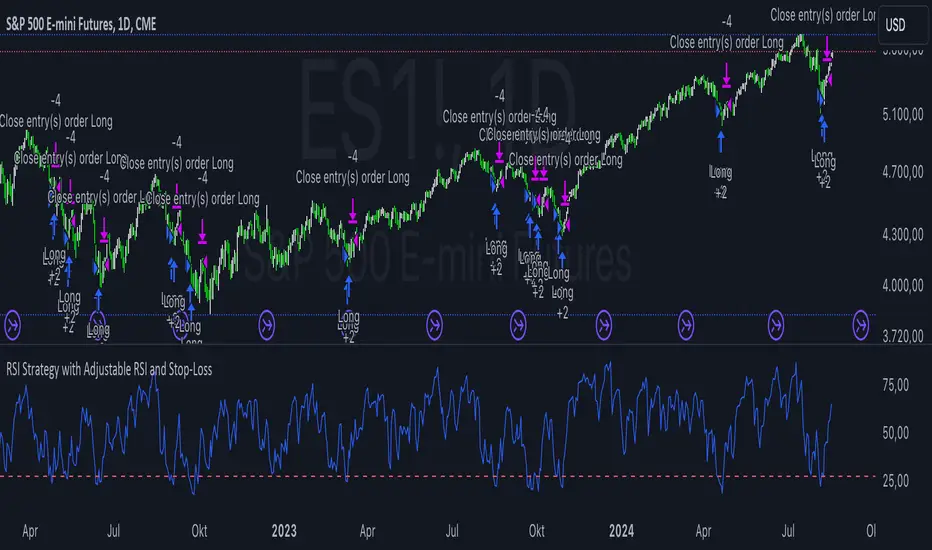
Double Bottom and Top Hunter### Türkçe Açıklama:
Bu strateji, grafikte ikili dip ve ikili tepe formasyonlarını tespit ederek otomatik alım ve satım işlemleri gerçekleştirir. İkili dip, fiyatın belirli bir dönem içinde iki kez en düşük seviyeye ulaşması ile oluşur ve bu durumda strateji long (alım) işlemi açar. İkili tepe ise fiyatın belirli bir dönem içinde iki kez en yüksek seviyeye ulaşması ile oluşur ve bu durumda strateji short (satış) işlemi açar.
- **Dönem Uzunluğu ve Geriye Dönük Kontrol:** Strateji, varsayılan olarak 100 periyotluk bir zaman dilimini temel alır ve bu süre boyunca en düşük ve en yüksek fiyat seviyelerini belirler. Geriye dönük kontrol süresi de 100 periyot olarak ayarlanmıştır.
- **İşlem Açma Koşulları:** İkili dip tespit edildiğinde long pozisyon, ikili tepe tespit edildiğinde short pozisyon açılır.
- **İşlem Kapatma Koşulları:** İkili dipte, en yüksek seviyeye (HH) ulaşıldıktan sonra fiyatın daha düşük bir seviye (LL) yapması durumunda pozisyon kapanır. İkili tepede ise tam tersi bir durumda, pozisyon kapanır.
- **Zigzag Çizimi:** İkili dip ve tepe formasyonları, grafik üzerinde yeşil (dipler) ve kırmızı (tepeler) zigzag çizgileri ile gösterilir.
Bu strateji, özellikle 1, 3 ve 5 dakikalık kısa zaman dilimlerinde yüksek başarı oranına sahiptir ve piyasadaki kısa vadeli trend dönüşlerini yakalamada etkili bir araçtır.
### English Explanation:
This strategy automatically executes buy and sell orders by detecting double bottom and double top formations on the chart. A double bottom occurs when the price reaches a low level twice within a specific period, prompting the strategy to open a long (buy) position. Conversely, a double top forms when the price reaches a high level twice, leading the strategy to open a short (sell) position.
- **Period Length and Lookback Control:** By default, the strategy is based on a 100-period length, during which it identifies the lowest and highest price levels. The lookback control period is also set to 100 periods.
- **Entry Conditions:** A long position is opened when a double bottom is detected, while a short position is opened when a double top is identified.
- **Exit Conditions:** In the case of a double bottom, the position is closed after the price reaches a higher high (HH) and then makes a lower low (LL). For a double top, the opposite occurs before closing the position.
- **Zigzag Plotting:** The double bottom and top formations are visually represented on the chart with green (bottoms) and red (tops) zigzag lines.
This strategy is particularly successful in short timeframes such as 1, 3, and 5 minutes and is an effective tool for capturing short-term trend reversals in the market.